That Feeling
Several weeks ago, while writing up a nice set of results that extended some work I did last year, I found that I was stuck finding the right wording for how I should nuance a (seemingly minor) matter in the introductory remarks. It was partly because, frankly, I’d got bored of the standard introduction I usually make to papers on this particular subject (matrix models and 2D gravity), because I’ve written quite a few in the last two years (10-Yikes!). But I’d found a new feature that warranted a more careful way of saying the usual things, and I wanted to incorporate that aspect, and also get the Reader interested in why this aspect was interesting and worth unpacking. I played around with better ways of saying it, and still was not entirely happy. I chipped away for a bit more over a few days, and kept coming up with something less than satisfactory. I’d carry on with things in the body of the paper that would be there whatever the introduction said. Then, after coming back to the introduction and trying again, I had to stop and explore the consequences of some of the rephrasing I was doing – to make sense of the new way I was trying to say what I wanted to say.
And then it happened…
You might know that feeling: A sort of pop goes off in your head and a tingle through the whole body, and then everything looks different all of a sudden, because you realize that you’ve found a completely new way of looking at things. A way that fits *so* well and incorporates so many of the facts that it just. feels. inevitable.
That’s what happened. And then I tried to see what it would say about the larger picture of physics this all fits in, looking for a way to make it fit, or to challenge the idea to see if it breaks. Not only did not not break, it just kept making sense, and (almost like the idea itself took charge of the process) immediately offered solutions to the problems I threw at it, and readily gobbled up existing challenges that the community has been facing for a while, and explained certain things that have been a puzzle for a long time.
For the next few days I actually could not write properly at the keyboard any more. My hands were trembling every time as I utterly rebuilt the entire paper and my world view, and I could barely sit still at times.
I know this sounds like a lot, and you should know that I am open to the possibility that it is somehow wrong, but it is too compelling not to share, so that’s what my paper that came out earlier this week is all about. I am not going to repeat the paper here, but will try to highlight some features of it that form a foundation for why this changes a lot about how we think about things in this corner of physics.
Random Stuff
Let me start in the simplest way possible, as I have done in the past, with a model that is well known to many different physics communities. The Gaussian random matrix model. Random matrix models have a very long history in trying to understand complicated systems (going back to Wishart (1928), and then Wigner (1955) – physicists seem to always forget to mention Wishart, and I’m sure I’m forgetting someone else too), and they show up in all kinds for systems. There are a lot of powerful results that have been developed, and you’ve read my writings about them here to do with how they get used for understanding aspects of string theory and quantum gravity in 2D, and also in higher dimensions. The “double scaling limit” is something I’ve talked about a lot here in particular. I won’t repeat all of it here, but invite you to go and look at other posts.
For definiteness, start with a model of 


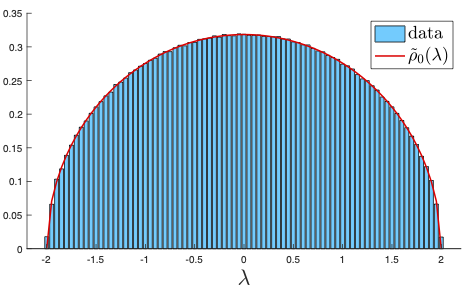
Wigner’s semi-circle law
For doing 2D quantum gravity, you can do a similar thing but the quadratic in the exponential (giving the Gaussian) is replaced by some more general polynomial. But for illustration purposes, this will do. (The Gaussian case gives something that’s better called topological gravity, but let’s not worry about why right now.) Things proceed from here by describing the eigenvalues with a smooth function – smooth because at large 
The double scaling limit amounts to scaling in to an edge of the distribution as 

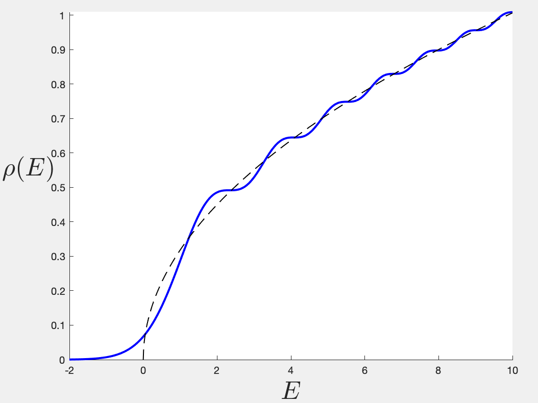
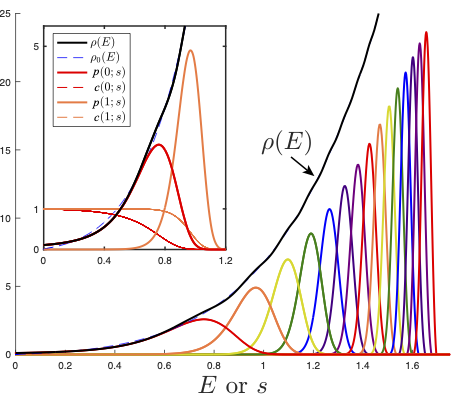
Full spectral density for the Airy model. Dotted line is leading perturbative part.
The zoom-in shows that Wigner is only correct to leading order, and there are corrections that show that there’s some leakage past the naive endpoint of the distribution (now located at 
The core thing I want to say is that in using matrix models for quantum gravity, and particular for string theory, starting in the late 80s and early 90s, some marvelous things came about – exactly solvable models of how to sum over all the contributions of gravity on surfaces of different geometry and topology, and in fact to go beyond the sum and capture physics that is “non-perturbative” in the expansion parameter (that counts topology: it is that
So here’s really the most key thing:
The Smash and Grab
I’ve been thinking for some time now that what actually happened around the time of the double scaling limit was a bit of a smash-and-grab. We (the string community) came into the random matrix model tool shed, found some really powerful tools and toys that we could see would be useful, and we went off and used them and built a powerful narrative around them. But we only grabbed things we kind of liked the look of, and there were a ton of other things left in the tool shed that went ignored because we either did not like them, or could not make sense of them in the moment. And we largely never went back for almost 30 years. In those 30 years, many of the tools continued developing, and in particular the ones we’d never really taken much interest in continued to develop further and in some really interesting directions. (Before some people get themselves too exercised over the use of the term “smash and grab”, I don’t mean it disparagingly. It’s just a turn of phrase. In reality, scientists borrow and lend tools and techniques all the time across the arbitrary divisions between sub disciplines. The toolshed was left unlocked, with a sign saying “please take what you want”.)
So what is the distinction between what we grabbed and what we left? It largely comes down to t’Hooft vs Wigner. When large
Well, off you go from there to the double-scaling limit which tells you how to tune the models to pick out smooth surfaces of those different topologies and the magic happens and you never look back. There’s some interesting words bolted on about non-perturbative corrections and instantons, and large orders in perturbation theory, and D-branes, and so forth. The leaking to the left in the figure above is discussed in these terms, and it is not wrong – just incomplete as we shall see. It’s nice stuff, don’t get me wrong. But that’s mostly all we do! From that perspective, the solid blue curve I drew above, which contains the all orders and beyond contributions to
Actually, it’s just beginning. Job just begun. The key point here is that there’s an underlying smooth spacetime intuition going on, and it makes it hard to let go when trying to understand much more. But there’s so much more, and the way to get at it is through Wigner, who kicked off all this in the first place, but not for the purposes of studying smooth geometry. He was not thinking about smooth stuff that eventually gets a gravity interpretation. He was thinking about combining spectra of many Hamiltonians into one model that can tell you about properties shared by the ensemble of spectra. He started doing this for nuclear physics, but the spirit of it is in many other fields such as the theory of disordered systems. You might want to study this particular complicated thing in your lab, but it is hard. So you study a model of the whole family of systems to which that thing belongs, and if you’re lucky, and do it the right way, the theory will tell you very specific things about how the family works, and indeed give you some very useful information about the complicated thing in your lab at the end of the day. (I say this now because os something I’ll come back to in a while.) So the main point is that the stuff to do with statistics and averaging over spectra has a massive set of powerful tools associated to it too, but we left those on the table. In a way, they lie at the roots of the whole enterprise, and are way older that the t’Hooftian tools we chose to play with.
What I realized in that moment of clarity I referred to above was simply the full implications of putting the Wignerian approach right alongside the ‘t Hooftian approach, and when you do so, it changes how everything looks. It all began already with things I talked about here on the blog back in May of last year, and it is really clear when you study actual matrices and just do the experiment. (I highly recommend it. I tell you how in various footnotes in the paper.)
If you zoom in on the density’s edge with all the corrections you get this:
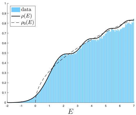
which is maybe not too surprising. It’s just the histogram zoomed in. What’s the big deal?
Ok. How about in your histogramming you label whether a matrix’s eigenvalue is the largest, next largest, etc in the list, and then color code the histograms of them… so all lowest ones are red, all next lowest are orange, etc. Now let’s draw it again:
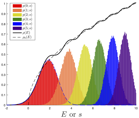
Oh. And it is usually at this point (since Spring last year and ever since then even though I’ve been showing it to people and have written papers about it) that I get silence from even some of the most seasoned matrix model persons (on the gravity side). You see, in the field we talk a lot about bumps in the spectrum due to (a hand waves vaguely) non-perturbative effects, but we usually don’t go much further than this. The point is that this is the origin of the bumps. (I hope that you maybe can see by eye that if you add the individual histograms together, you’ll rebuild the full
And once you see this, and really look at it, you can’t unsee it.
Statistics
Well, if you show this to people in the random matrix model community that cares more about statistics and disordered systems and the like, they know what this is immediately. They can compute these curves (with difficulty, but straightforwardly nonetheless) using tools the gravity/string community left on the floor of the tool shed way back when when we did the “smash and grab” 30 years ago!
The first one, the probability distribution of the lowest energy level, is actually now a celebrated probability called the Tracy-Widom distribution. Guess when it began to be fully appreciated in the random matrix literature? 1993/1994, just after we gravity folks had lost interest in matrix models, and gone off to do other things!! (Wonderful things, mark you.)
Tracy-Widom shows up in a wide variety of physics and mathematics problems, and is anticipated by many to be maybe as important as the normal distribution is, for a large class of systems – In other words, arising in a universal way when certain basic conditions are met. (See a piece here about it.) It emerges here by computing a certain mathematical/physical object called a “Fredholm determinant”, and you can learn more about the technique (with references) in my paper. (Gaudin showed they can be used for this purpose as far back as 1961! That’s how old this wonderful stuff is.)
The point is, if you can fully write down the right key players in the matrix model (and my approach shows how to do that for that for models that define various JT gravity models of interest – see several earlier posts), then you can build the Fredholm operator and compute its determinant at every point on the energy line, and with some manipulation, turn it into the probability for the lowest energy level, for the next lowest, the next, and so forth. I’ve gotten fairly adept at doing this now (using wonderful methods developed by Bornemann) so here are the first 15 levels for the Gaussian/Airy model:
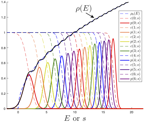
Airy model’s peaks computed using Fredholm Determinants
So as I said: once you see this, you can’t unsee it. The point of view of the gravity theorists that centers the “spectral density” 
JT gravity microstates from Fredholm determinant techniques
Look at those peaks. Take either their means, or the tops of the peaks (it does not matter which right now, for making this central point – I’ll come back to this below). This picks out a single energy associated to each peak, giving the ground state, the next level, next, etc. This is what the typical matrix is doing! We can’t ignore this information (although we have been doing so all along). The spectrum is therefore actually widely spaced, and as you go to higher energy (where people do perturbation theory, and where ‘t Hooft reigns) the spacing becomes smaller, until in the limit where people have studied JT gravity using other techniques, and know it best, indeed the spectrum is continuous… but at lower energy it becomes discrete, in a very definite manner. My conjecture is that it is a spectrum like this that constitutes the full quantum description of JT gravity.
I also think this this is not just about JT gravity. It is about a much wider family of 2D gravity theories that matrix models can capture.
Controversial
Anyway, that’s those are the core ideas. It is massively controversial, I know, since I am saying that the claim that JT gravity is fundamentally an ensemble is not correct. Instead there is a specific Hamiltonian with a definite spectrum for it, and the ensemble physics (the matrix model) is yelling at us to notice it. It contradicts claims in the literature that say otherwise, but I think there could be a loophole in the currently accepted reasoning. I am not saying that I’ve found a proof, but I think we now have a super-clear suggestion that I think can be verified using other techniques now we know it is maybe there.
I’m also saying that I’ve found a way out of the factorization puzzle in AdS/CFT in all dimensions (a large program of activity right now), since JT gravity now has a more traditional holographic dual: it is a (new?) type of quantum mechanical theory that has a discrete spectrum that becomes the continuous (Schwarzian) form only at large 
I’m also saying that all matrix models that we’ve been using in the service of models of 2D gravity (not just JT gravity) have not been fully interpreted for their full content, and in each case there is a sort of baby holography of the kind I just described going on.
I’m also saying something very nice about the spectrum of low temperature black holes in higher dimensions, from which JT gravity emerges as a model of that sector. I’ll expand upon that another time (see paper).
And I say a lot more in the paper, including describing how combinations of ‘t Hooft and Wigner are responsible, within the matrix model, for giving smooth surfaces on higher topologies, and that’s how they actually yield gravity on higher topology, and physics that is non-perturbative in topology. I think this is how it works in higher dimensions too, although this is harder to demonstrate fully.
A nice thing about this is that even if people don’t like the idea that there’s a single hamiltonian, and all that implies, they still have to accept that there’s a massive amount of information in the matrix model that we’ve all been ignoring for a long time. Those peaks play no role in the standard picture of how matrix models and gravity work. And they aren’t a minor detail, but in fact underlie the whole picture. So, as I said, they can’t (or at least) shouldn’t be unseen, now that they have been seen.
I will say more some other time, I hope.
-cvj
(P.S. There is the issue (that I thought long and hard about for some weeks) as to whether the true spectrum is found by taking the tops of the peaks or the mean of the peaks. I chose the mean in my paper mostly based on making contact with the results from the quenched free energy of the whole matrix model. In other words, the matrix model is pointing to the average energy. This also fits with results from a similar D-brane-like object in the theory that computes the average matrix spectrum. So that’s a pair of strong hints. But it is possible that it really is the tops of the peaks that determine the “true” spectrum. The most frequent energies of the ensemble. This would correct things slightly, but ultimately is less crucial to the main overall point being made – that there *is* a spectrum, pointed to by this analysis. A nice reason to focus on the tops of the peaks might be because that they represent a special phase transition, or at least crossover between two kinds of phases, in a dual system. I’ve been wondering if that might be relevant to the story.)
(P.P.S. If I’m quiet for a while, let’s hope it’s not because I’ve been taken out by the syndicate Big Matrix. 🙂 )

Pingback: A New Distribution | Asymptotia
Mitchell:- Indeed! We shall see down the line (I hope) what this might all lead to! There are some rather interesting new types of universality at play in all this.
–cvj
I notice you mention the Marcenko-Pastur distribution. The first time I ever heard of this, was in a theory of phase transitions in deep learning networks (1810.01075). It would be rather amazing if some of these considerations about geometric vs non-geometric phases, actually helped us understand AI too.
Thank you Nikolay! Yes, I’d forgotten much of that fun N=2 stuff. Thanks for the reminder!
Thanks for the nice and clear summary and congratulations on the paper! This story reminds me of another holographic example (which you know well!) where the Wigner semi-circle law emerges. See this wonderful paper for more details https://arxiv.org/pdf/1302.6968.pdf . Of course the setup is very different since, amongst other things, here one varies a coupling and not energy.