Completing a Story

[A rather technical post follows.]

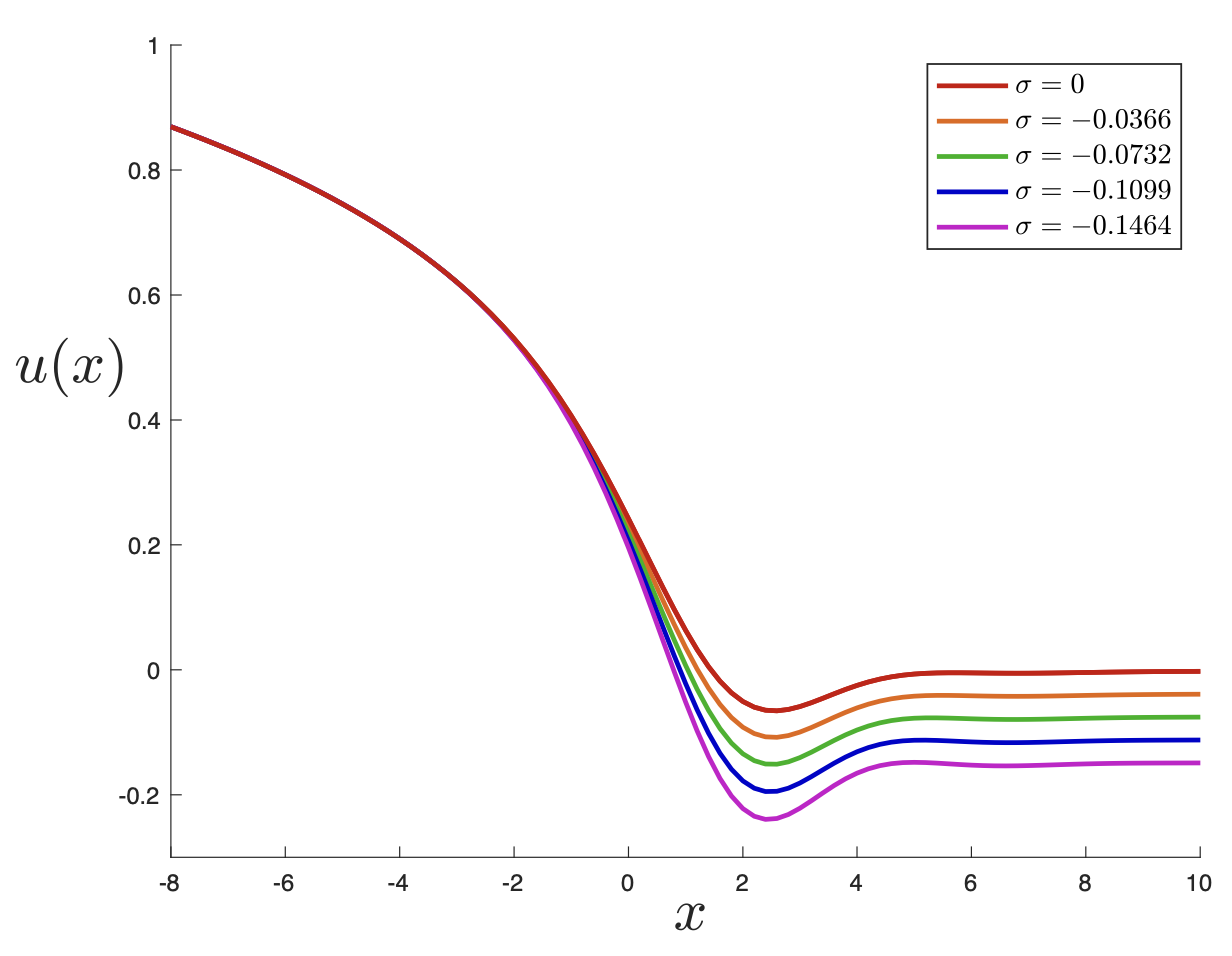
This figure will make more sense later in the post. It is here for decoration. Sit tight.

For curious physicists following certain developments over the last two years, I’ll put below one or two thoughts about the new paper I posted on the arXiv a few days ago. It is called “Consistency Conditions for Non-Perturbartive Completions of JT Gravity”. (Actually, I was writing a different paper, but a glorious idea popped into my head and took over, so this one emerged and jumped out in front of the other. A nice aspect of this story is that I get to wave back at myself from almost 30 years ago, writing my first paper in Princeton, waving to myself 30 years in the future. See my last post about where I happen to be visiting now.) Anyway here are the thoughts:

Almost exactly two years ago I wrote a paper that explained how to define and construct a non-perturbatively stable completion of JT gravity. It had been defined earlier that year as a perturbative series in a landmark paper by Saad, Shenker and Stanford (SSS), through an equivalence to a matrix model. Six months later I showed how to extract tons of explicit non-perturbative results from my definition, computing physical quantities that simply weren’t computable before. (And did it for several super JT models too.)

[Perturbation theory here means order by order in a parameter that counts the topology of the two-dimensional geometry of the gravity theory. And by the way, I wrote a couple of posts with background on all this here and here, as well as a more recent one here. Somehow I managed to not get around to writing about the 2019 paper itself it seems, nor have I written about the newest results involving Fredholm determinants that I’ve been quite taken with. That last ended up being a PRL (funny story, must write about it at some point) and I will be writing a big paper about how it all works soon.]

[As an aside, I do find it a bit dismaying that many people will still rather get themselves all contorted into knots than accept (and even acknowledge the existence of, in some prominent cases) that this is a legitimate completion of the theory, with a lot of content highly relevant to what they themselves are working on. Had the same work been done elsewhere and/or by others, I’m fairly quite sure it would have had a different reception by now. But over the many years I’ve got used to the tacit assumption by many of even my most well-meaning colleagues that I can’t possibly really have done anything important.]

An interesting question I commonly get is whether there could be other completions besides the one I found. Sometimes this question is code for “surely someone else, meaning not you, will soon produce the correct completion”, but sometimes it is out of genuine interest, so I try to interpret it in that latter spirit. A followup set of questions I’d add to that is: How different can two completions be? Are there universal features we can learn? What would be criteria for picking one as correct over another? Etc. All very interesting indeed.

So are there other completions currently? The answer is no. Not one. There have been some interesting suggestions, starting with one in SSS’s original paper. Earlier this year, Gao, Jafferis and Kolchmeyer expanded upon SSS’ suggestion somewhat. But there’s no actual computation of non-perturbative results. Those nice ideas are manifestos for a completion, which is not the same as an actual completion.

But it is possible that one day they, or someone else, might be able to turn the suggestion into a working computational toolbox that yields answers for the non-perturbative physics. It is also possible that some other approach will produce an alternative answer. So how do we cross-compare, and what criteria do we use?

Well, that’s part of the point of the paper. A framework is needed, one that is itself intrinsically non-perturbative. One that uses variables that can reach beyond geometry. I set out to lay out how such a framework all works as clearly as possible. It’s one we already know! The matrix model (but built in the way I do it, not the perturbative way).

The bottom line is that there is a remarkable and robust dictionary between the matrix model and the gravity model, order by order in perturbation theory. You ask what the result is on surfaces with 5 handles, and you can compute it using the gravity path integral, and a completely different computation gives you the same answer using the matrix model. But the matrix model effortlessly – if you use the framework I’ve been trying to get people excited about for two years – allows you to compute results not just in perturbation theory but beyond. So why not use the variables the matrix model naturally supplies to phrase the questions about non-perturbative physics? The formalism is crying out that these are the right tools, so why not use them?

Slightly less abstractly (but still a bit abstractly since I am not going to rewrite the paper here) everything ultimately follows from the existence of a variable, , which lives on the real line, and a function of it, . All the physics turns out to be defined in terms of combinations of quantities that follow from knowing , inheriting some dependence on , which are then integrated over from to some value (which for JT gravity is actually equal to zero).

(For reasons I won’t go into here (but it is a beautiful story that’s key to the discussion) the region with between and is the Fermi sea of a fermionic many-body construction that underlies the whole system, where is the Fermi level. The integrals build properties of fermionic many body states that describe the physics. They are simply a continuum version of summing over all the energy levels up to the Fermi level.)

The Fermi sea and beyond

Simply put, working in perturbation theory amounts to having only specified order by order in perturbation theory in the region of large negative . 99% of the literature to date on JT gravity has been equivalent to working in this regime! The job of understanding the rest of the theory (at least as a matrix model) is go beyond this, and know the full story for in the region of integration. Once you know the origin of all these quantities it is super-clear that the most natural way to understand the full story of is to understand it as a function on the whole real line. So not just the region with between and but also what I call the “trans-Fermi region” from to . This is not fanciful, but is what the matrix model tells you: The function is incomplete without all the data about it specified along the whole real line, and all of this feeds into the physics.

Being able to discuss properties of in the trans-Fermi region is the natural way to discuss properties of the non-perturbative physics. It is then an easy next step to ask
what possible behaviour can have. The “Consistency Conditions…” of the title of the paper is simply a short list of reasonable conditions you can place on , including things like continuity (as you go from Fermi sea to trans-Fermi regime), and so on and so forth.

The core point is that this is a proposal for a framework for discussion of other completions as they come on the market. It works as follows: If you have a different method for computing the perturbative expansion of JT gravity, you are either implicitly or explicitly defining the same function and variable , and it must agree with the one already described above. Now let’s say your method also defines a non-perturbative completion of the expansion too. Then it implies information about the full , in the Fermi sea for sure, and possibly also in the full trans-Fermi region too. Comparing the results of your completion to mine or anyone else’s completion is simply a matter of comparing the different functions since all the physics follows from that one function. Simple. (Although of course extracting the implied might not be easy to do in all cases, but it must exist.)

Here’s a bonus thing: In formulating the consistency conditions I realized that my completion of 2019 is in fact part of a family of completions! This is great since it provides a lovely example of what I set out for: A framework within which one can compare different completions. So I set about comparing them, starting with their different functions. The case was my 2019 completion. There’s a tightly constrained range of them (that I work out) parameterized by . The figure at the very top shows some samples.

Here’s another bonus thing: Turns out that the framework (and the nature of the continuous family of completions I found) has a lovely string theory language underlying it that makes everything quite natural. The formalism easily adds physics corresponding to certain spacetime boundary conditions known as End-of-the-World branes in this language because they are just D-branes that I’ve known how to add to this theory since 1992 (back even before they were called D-branes). So a lot of the apparatus that makes this all run like a well-oiled machine was something I helped develop 30 years ago, and in fact, showed the full understanding of in my first paper as a postdoc, written when I was in Princeton.

It is a lovely and beautiful story involving certain modified Virasoro constraints, tau-functions, boundary cosmological constants, integrable systems, and so forth. It’ll have to wait to be told here as I’ve another paper to write.

Also, I must cook dinner.

–cvj