(A somewhat more technical post follows.)
Continuing from part I: Well, I set the scene there, and so after that, a number of different ideas come together nicely. Let me list them:
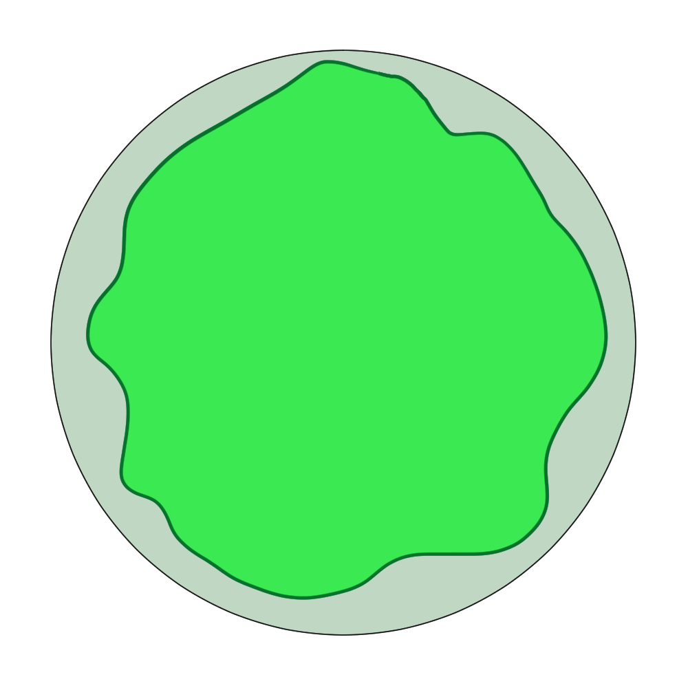
What “nearly” AdS_2 looks like via JT gravity. The boundary wiggles, but has fixed length 1/T.
- Exact solution of the SYK model (or dual JT model) in that low temperature limit I mentioned before gave an answer for the partition function
, by solving the Schwarzian dynamics for the wiggling boundary that I mentioned earlier. (The interior has a model of gravity on
, as I mentioned before, but as we’re in 2D, there’s no local dynamics associated with that part. But we’ll see in a moment that there’s very interesting stuff to take into account there too.) Anyway, the result for the Schwarzian dynamics can be written (see Stanford and Witten) in a way familiar from standard, say, statistical mechanics:
, where
is the spectral density of the model. I now need to explain why everything has a subscript 0 in it in the last sentence.
- On the other hand, the JT gravity model organises itself as a very interesting topological sum that is important if we are doing quantum gravity. First, recall that we’re working in the “Euclidean” manner discussed before (i.e., time is a spatial parameter, and so 2D space can be tessellated in that nice Escher way). The point is that the Einstein-Hilbert action in 2D is a topological counting parameter (as mentioned before, there’s no dynamics!). The thing that is being counted is the Euler characteristic of the space:
, where
are the number of handles, boundaries, and crosscaps the surface has, characterising its topology. Forget about crosscaps for now (that has to do with unorientable surfaces like a möbius strip
– we’ll stick with orientable surfaces here). The full JT gravity action therefore has just the thing one needs to keep track of the dynamics of the quantum theory, and the partition function (or other quantities that you might wish to compute) can be written as a sum of contributions from every possible topology. So one can write the JT partition function as
where the parameter
weights different genus surfaces. In that sum the weight of a surface is
and
since there’s a boundary of length
, you may recall.
The basic Schwarzian computation mentioned above therefore gives the leading piece of the partition function, i.e.,
, and so that’s why I put the subscript 0 on it at the outset. A big question then is what is the result for JT gravity computed on all those other topologies?!
- In seemingly unrelated developments, it had been noticed (from studies of SYK as a quantum chaotic system – see Garcia-Garcia et al, Cotler et. al., and Saad et. al.,) that the spectral density has certain features reminiscent of random matrix models. (In fact, this is part of a more general discussion of quantum chaos and matrix model statistics, and my goodness, it seems I’ve written a post about this 14 years ago, so go there for more, with refs.) For example, the energy levels tend to not want get too close to each other, almost as though they are repelling each other. In random matrix models, the energy levels are eigenvalues of the random matrices, and the eigenvalue distributions show the same features. In fact, at large
(the size of the matrices) this feature is responsible for being able to write the density as a smooth function.
- But there’s another aspect of matrix models that is of relevance here, emerging from studying toy models of QCD (the strong interactions). Treating them as toy field theories, where the basic field is the matrix
, you can go ahead and do what you’d normally do in field theory, which is to work out the Feynman rules for diagrams representing interactions. Following ‘t Hooft, the propagators and vertices you’d draw are made of thickened lines, or ribbons, in order to keep track of the two indices of the matrix
,
and results are weighted by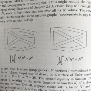
Two sample ‘t Hooft-Feynman graphs. One can be drawn on a sphere, the other a torus. (Click for larger view.)
, where
is the Euler number of the surface the Feynman diagrams that gave the result can be drawn on. At this point I was going to draw you a diagram or two when I recalled that I’ve taught this stuff M times, for M large, and at some point I’d put it into a book (D-Branes (2002), see chapter 18). So see (enlarge-click) the photo on the right. The example there contrasts the sphere and the torus. Vertices contribute
- Well, this is looking a lot like the two dimensional quantum gravity setup described a bit earlier, right? And yes, there’s a long history of studying 2D gravity using matrix models! This work was mostly motivated by the fact that it is also a model of the world-sheet expansion of string theory, but also because it is a very solvable model of a quantum gravity, where the spacetime splits and joins (changing topology) as ought to be possible somehow if you let gravity (the dynamics of spacetime) be truly quantum, (in some sense of the word “quantum” anyway). When life hands you a solvable model of something that you’re wondering about in principle (e.g., quantum gravity in 4D), you take it and learn what you can from it that might tell you about the real thing you’re interested in.
Well, it is one thing to guess that maybe there is some large
and try to guess from its functional form what kind of matrix model it came from. Once you’ve made the guess of what kind of double scaled matrix model it is, you can then check that the higher genus contributions on both sides of the equation (JT gravity = matrix model) agree. For all genus,
. There are an infinite number of genera
, so given that you’re working in finite time, you’d better have powerful relations that connect results from one value of
. (It might also be useful to either be, or to team up with, a grandmaster of the field whose kung-fu is strong, having co-discovered and developed a lot of this technology before, as well as looking out for new tools from mathematics and other fields that can help.) So yes, that’s what Saad, Shenker, and Stanford did. The primary starting point is that this is not just going to be a large
- So what’s the double-scaling limit? Let’s take a look at some diagrams from a matrix model again. These ones were drawn from some notes I made way back in 1998. (Etudes on D-Branes )
As you can see from the picture with the dotted lines, every diagram you draw can be mapped to a tessellation of the surface that it can be drawn on. In the example on the left, I’ve broken the sphere up into 1 square and 6 triangles. (I’ve left the torus diagram on the right as an exercise.) Now, that’s the sphere topologically, but as a smooth approximation to a sphere, it is pretty rough. What you want is to have (for a given fixed size sphere) a tessellation made out of lots of polygons, or, put differently, a ‘t Hooft-Feynman diagram made of lots of vertices. The more polygons, the better the approximation to a smooth surface. So this is what the double scaling limit is all about. It tunes the couplings in the model’s potential to a point where such “large” surfaces dominate (in fact they diverge in the sum) and then rescales to make them finite size, sending rough tessellations like the one I drew above to zero size, contributing nothing to the final answers in the limit. In this way, you get a matrix model that has a genus expansion over 2D smooth surfaces – a 2D gravity theory. That’s the double scaling limit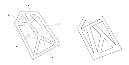
Drawing the “dual” to the t’Hooft-Feynman diagrams produces a tessellation of the surface on which they can be drawn. There’s a typical size of the polygons of the tessellation for a given potential.
There are many ways of doing this, corresponding to many different kinds of 2D gravity theory (for example, coupled to different kinds of 2D fields), so SSS had to piece together what kind of matrix model could give them the particular character of JT gravity. Many years of study of this kind of setup showed that the spectral density of such models have a particular character to them, and this was a major clue for SSS.
- (By the way, go and read some of the things I said in those notes 22 years ago about how I thought matrix models may well come back and be useful for teaching us about grown up gravity. For example, those thoughts about finding a way to first go off conformality in the gauge theory in order to define a double-scaling limit seem very relevant now…)
- So, anyway, SSS began to look at the behaviour of Hermitian matrix models in the double-scaling limit in order to use them as the building blocks of the JT gravity matrix model. But instead of having the spectral density of the old Hermitian matrix models, it has the spectral density computed by the Schwarzian action, that I mentioned above (but did not show explicitly). They cleverly build the leading order (in genus expansion) behaviour they need and then using some very powerful recursion relations (by mathematicians Murzakhani, and by Eynard and Orantin) define the entire perturbative expansion for all genus. There’s a ton of ideas and computations I’m leaving out here, but the point of this post is to give you the general idea of what’s going on, not to reproduce their paper – you can just read it.


Anyway, that’s the story so far. Now I can tell you what my paper Non-Perturbative JT Gravity is about! But this post has gone on a bit long, and I’ve other things to be getting on with, so I’ll delay until part III. But you can guess, maybe, from the title, and if you’ve read other posts of mine here about string theory perturbation expansions: There should be more than just the sum over all genus. What about the non-perturbative sector?
See you later.
–cvj
