(A somewhat more technical post follows.)
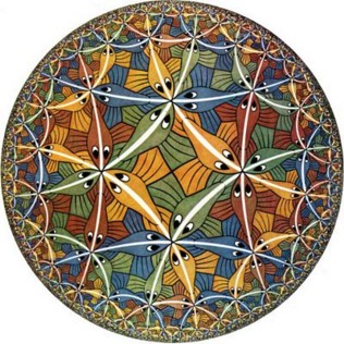
Escher’s “Circle Limit III”, nicely illustrating (Euclidean) AdS_2 for us.
JT gravity is a model of two dimensional gravity that goes back many decades. But there’s not much going on in 2D (or (1+1) dimensions, one space and one time), I hear you cry! Well, nevertheless this turns out to be a very useful arena for studying very important quantum key properties of black holes in more realistic dimensions. Let me take a step back to unpack that.
There is a long tradition (which you might know about) of studying models of black holes in string/M-theory, in different limits and approaches, each with their own advantages and disadvantages. The simplest models are often too simple to capture some of the important features of black holes, and some models get nicely at certain aspects while having little to say about others. And of course, some of the more realistic (but still simple) black hole models are still too complicated to be directly solvable in order to reliably explore phenomena of interest.
I’d say that a certain class of models that has been discussed a lot recently has something new to offer. The prototype is something called the SYK model (Sachdev-Ye-Kitaev). It’s an even more crazy sounding starting point than 2D gravity, as it is a 1D model. There’s no space at all, just time: It is a model in (0+1) dimensions, if you like. It’s a special model of quantum mechanics, actually a bunch of 


Well, I heard people mention the SYK model increasingly over 2015 but I was thinking about too many other things (and was mostly dealing with being mostly sleep-deprived as a new dad), and so did not really pay much attention. Bandwidth issues, we’d say these days. I was happy to declare “we’ve got some of our best people on it”, and continued chipping away on other things where I could. Then in December 2017 I found myself sitting next to David Gross on a flight to the East coast (long story I forgot to blog about), and he mentioned that he’d been really excited by the SYK model and maybe I should have a look, since there’s a lot there that I’d probably like. And *still* some time went by without me clearing up bandwidth to look at any of it.
Catch up began in the Fall of last year (2019), but only after similarly missing following what was going on in a related area: JT gravity. One way of thinking about how JT gravity enters the story is to simply state that it is a holographic dual of the SYK model, in the sense of AdS/CFT, where you have a gravity theory on one side, and it is dual to a (conformally invariant) non-gravitational field theory on the other side. The key thing is that the gravitational theory has one dimension more than the field theory. I’ve spoken of such things a lot here on this blog so I won’t review, but instead let you dig a bit and find things to read in the archives. (You could put AdS/CFT in the search window, or maybe start here.)
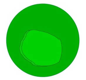
A ball showing the AdS/CFT setup. The interior has gravity on an anti-de Sitter spacetime, the the boundary has a dual (conformal) field theory.
Important technical note: In the setup I drew above, the metric which measures spatial distances makes spacings smaller and smaller as you move out from the center, approaching zero as you get to the edge. This is another way of saying that the distance to the boundary is actually infinite. There are famous depictions of all this in 2D – MC Escher’s tessellations of the Poincaré disc (where now time is treated as a spatial coordinate too – we work with “Euclidiean signature”). See “circle limit III”, at the top of this post, to the right. The fish get smaller as you move out, but they’re really all the same size, allowing MC to draw an infinite space in a finite bit of paper.
So here, the SYK model is like the Yang Mills theory and the JT gravity is like the AdS. Well, that’s not quite right, and in fact the “not quite” is what makes it interesting, for many reasons. First of all, we should really stick to low energies, where it turns out the SYK model looks more and more like a quantum mechanics with a conformal symmetry, so it is “nearly” CFT_1. If it were all the way exactly conformally invariant, you’d want to say it was maybe dual to AdS_2. But it isn’t, and instead is dual to something that is “nearly” AdS_2. And it is the JT gravity that gets the “nearly” to work properly in the following well-defined sense. It is a model of gravity with a special coupling to a scalar field (a dilaton-like coupling, if you are familiar with the term) such that the equations of motion for the scalar enforce (as though it is a Lagrange multiplier) that the overall spacetime curvature is constant and negative (as AdS_2 has), but there is an important boundary term involving the scalar too. When that is properly handled it tells you that the boundary is allowed to fluctuate in shape, but its length is fixed to be 
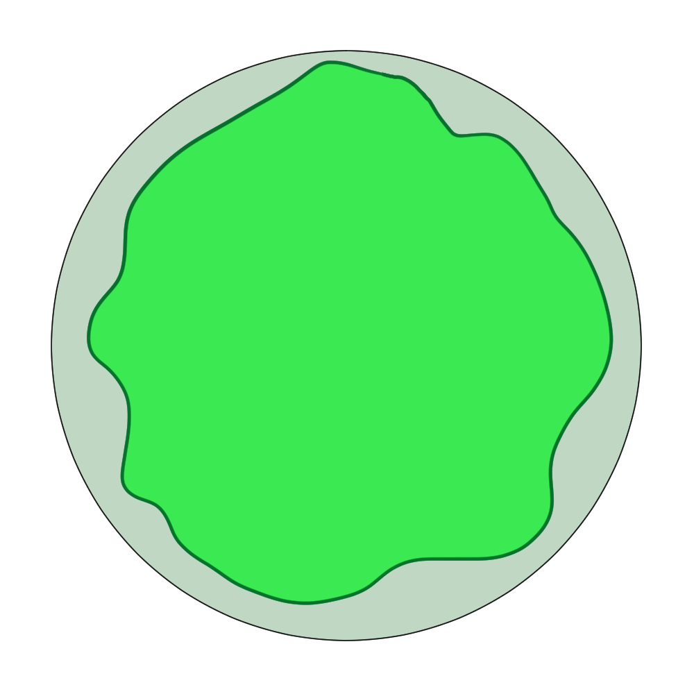
What “nearly” AdS_2 looks like via JT gravity. The boundary wiggles, but has fixed length 1/T.
 . (Notice that if the temperature goes to zero, then
  and so the whole thing heads toward being actually AdS_2, which makes sense.)
Actually, your statement at the beginning of this post that there’s not much going on in gravity in 2D is correct, and so there’s not much in the way of gravity to talk about until you couple it to something. Here it is coupled to the scalar field, and the interesting dynamics is really all about that wiggling boundary. Turns out that it is governed by a “Schwarzian” form (see e.g. the lovely papers of Jensen, and Maldacena-Stanford-Yang) that follows from the way in which the 
By the way, I’ve left out the names and papers of a lot more of the people who helped figure a lot of this out, but they are cited in my paper and the papers I cite there, so please have a look.
There are solutions of this 2D gravity model that can be interpreted as black holes in their own right, and there’s a lot of work on that, but it also describes black holes in higher dimensions (e.g., 4D charged or rotating), because the geometry near the horizon when the black hole is close to being extremal (so, at low 
(Historical note, for the younger ones reading (which might be all of you since no serious grown-up reads blogs, right? 😉 ): Some of us (myself included) spent years some decades ago back in the 1990s studying string theory background geometries corresponding to black holes where this kind of decomposition happens. E.g. 
(And by the way, JT gravity has been lurking in the literature since 1983/1984 – another great example of why its good to let people explore solid ideas even if they don’t immediately seem to have an application.)
In some ways, JT gravity is (part of) the answer for how to proceed beyond just the near-horizon geometry of a
Anyway, I think I’d better get back to other things for a bit. In part 2 of this, I’ll try to move the story forward a bit, including the part where I finally did pay attention to what was going on in this area, and discovered that things I’d been up to back in 1990 (!!), and that I’ve blogged about here a lot a decade or more ago, were highly relevant. In other words, I’d kind of been working on quantum black holes my whole career without realizing it!
-cvj

Pingback: Black Holes and a Return to 2D Gravity! – Part II | Asymptotia