[A somewhat more technical post follows.]
 So I have a confession to make. I started working on random matrix models (the large
Let me tell you a little more. You’re going to have to do some of the work and look at earlier things I’ve written for some of the background so that I don’t have to repeat myself. The starting point may well be my pair of posts entitled “Black Holes and a return to 2D Gravity”, Part I and Part II. There you will learn a bit about how the two-dimensional gravity theory called JT gravity is potentially useful for understanding the low temperature dynamics of more grown-up near-extreme black holes in (e.g.) the four dimensions we live in. Those dynamics are actually quantum dynamics. In other words, we’re learning something about a quantum description of spacetime physics that is close to what we care about in our world. (In brief: the zero temp 4D physics factors into a 2D gravity (AdS2) times a fixed two-sphere. Moving away from that limit is captured by the 2D theory known as JT gravity.)
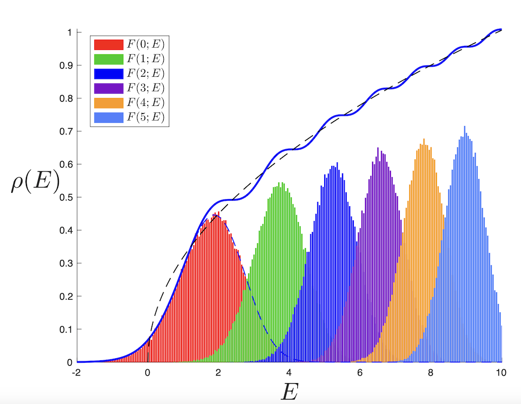
Anyway, I’ve been trying to get people to understand and appreciate more why we should all be excited about the matrix model description of JT gravity (and hence near extremal 4D dimensional black holes), particularly when you can get access to what I’ve called “non-perturbative physics”. Perturbation theory is a topological expansion in the genus or the 2D gravity surfaces here: They all have one boundary (periodic Euclidean time) and so you start with the disc and add handles, and possibly more boundaries, to compute your various physical results. But non-perturbative physics uncovers some very important features. Among those are the “bumps” in the spectral density of the theory. Here’s an example for a toy model called the Airy model (where the answer can be written analytically).
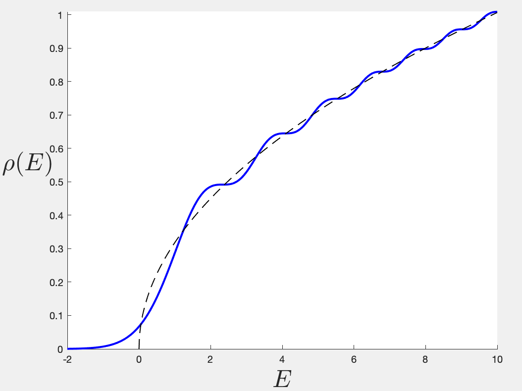
Full spectral density for the Airy model. Dotted line is leading perturbative part.
 In the figure, the dotted line is the leading perturbative piece – the disc order – which is
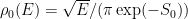


Well, those bumps are a sign of the underlying discreteness of the spectrum, and in particular, matrix model statistics is such that eigenvalues don’t like to lie near each other (in fact they repel) and so they spread out, taking up positions are on average nicely spaced from each other in any typical spectrum. My main point is that the map between matrix models and JT gravity, and JT gravity and near-extreme black holes, identifies the matrix eigenvalues with the black hole quantum micro-states.
Putting it more quantitively, recall that the topological expansion parameter, 


So anyway, to cut a long story short, much of my research last year was showing how to actually formulate the matrix model descriptions of several JT gravity variants such that one can actually uncover those bumps in the spectrum. And I succeeded in doing it for a variety of examples. (You can look here or at its companion – the pair were an editor’s suggestion in PRD, which was nice.) Many interesting features of the various results struck me as interesting, and so the natural question has been how best to understand the physics of these underlying micro-states that are revealing themselves? In particular, how does the thermodynamical description of the black holes, that we are pretty used to at high temperatures, extend down to lower temperatures when we must understand it in terms of the micro-states and their statistical properties?
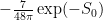
It is these questions that have been on my mind for a while, and the big specific question I’ve been asking (as have others, like Engelhardt et. al.) is: “How do you compute the quenched free energy of JT gravity?”. This is the quantity 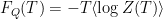


Free energy (annealed) for Airy model.
This just comes from working out that 

Well, my point, since a paper I wrote last August, is that the answer to the question about how to compute
But in any case, here’s my confession. Having finished the paper, I decided to take some time out from specific project work for a day or two, and decided to play (perhaps to some this is an odd bit of entertainment) with some random matrices for real, and build a concrete illustration of the often-said words (above) about the bumps in the spectral density showing properties of the underlying discrete spectrum. The idea is that an individual matrix would have a series of delta functions at the energies in the spectrum, but a given matrix randomly chosen might have its energies lightly to the left or the right of those of another member of the ensemble, so the delta-function spikes broaden out into peaks if you put all the spectra together. See this for real meant, as I said, that I sat down and generated random (Gaussian) 100 by 100 Hermitian matrices, (a couple of lines of code in MatLab) and worked out their eigenvalues (one line of code), and repeated thousands of times. Bin the eigenvalues with histograms and the famous Wigner semi-circle emerges quite readily for the shape of the distribution (takes less than a minute). Embarrassingly, I’ve never explicitly done this before! The next step was to focus attention on an endpoint of the distribution, and focus attention there while taking the scaling limit on the energies (zoom in by a power of
The Airy model spectral density with underlying microphysics statistics
There’s the famous “leaking out” of the eigenvalues from the semicircle edge into the negative 

So anyway, that’s my confession. I’d never done that hands-on exercise of sampling matrices before and it is so simple and (although I knew it “intellectually”) somehow illuminating. (The nature of writing online is that there’s going to be one or two readers already typing snotty remarks into the comments about how well-known and trivial this is. Good for them, those advanced beings. I never said it was hard or unknown, just nice to do.) I’ve had other experienced matrix model researchers tell me they also found it illuminating to simply look at these results. Sometimes we get so into the sophisticated methods that we forget to get our hands dirty with the basics.
So, well, this was such fun that I continued. You can make one change in the short computer program to build Hermitian matrices that have a positive spectrum (“Wishart” matrices they are often called: 
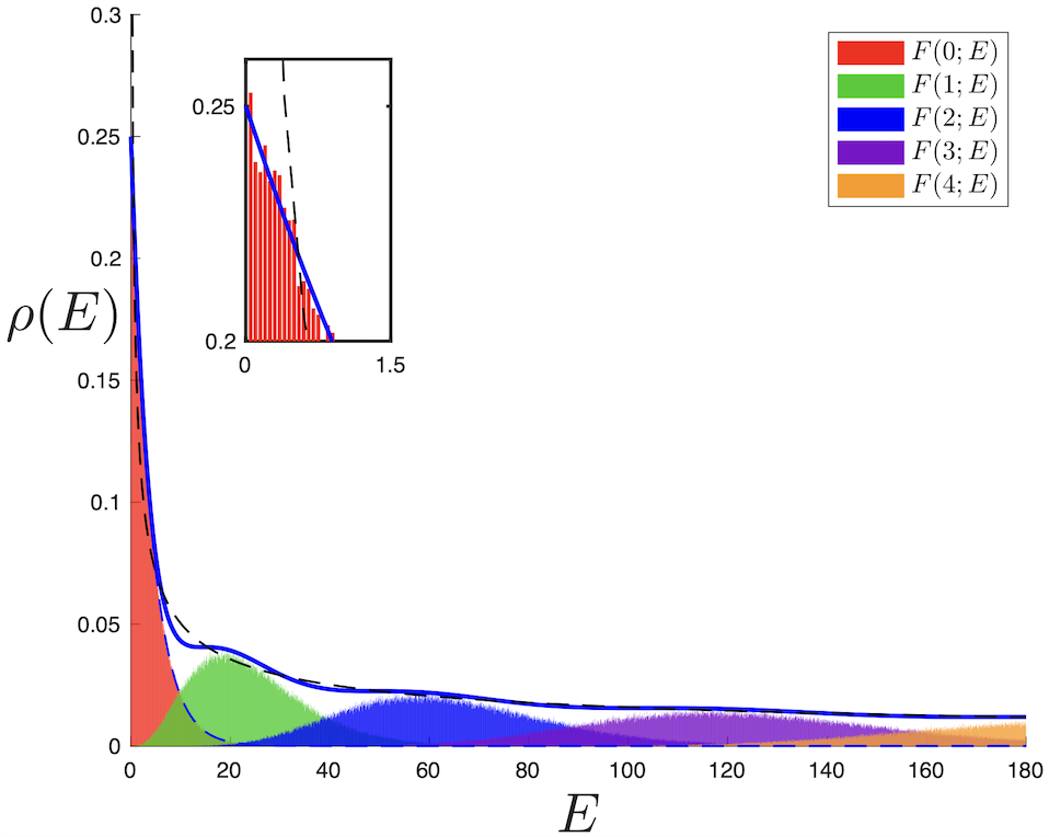
The Bessel model spectral density alongside some underlying microphysics
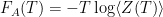
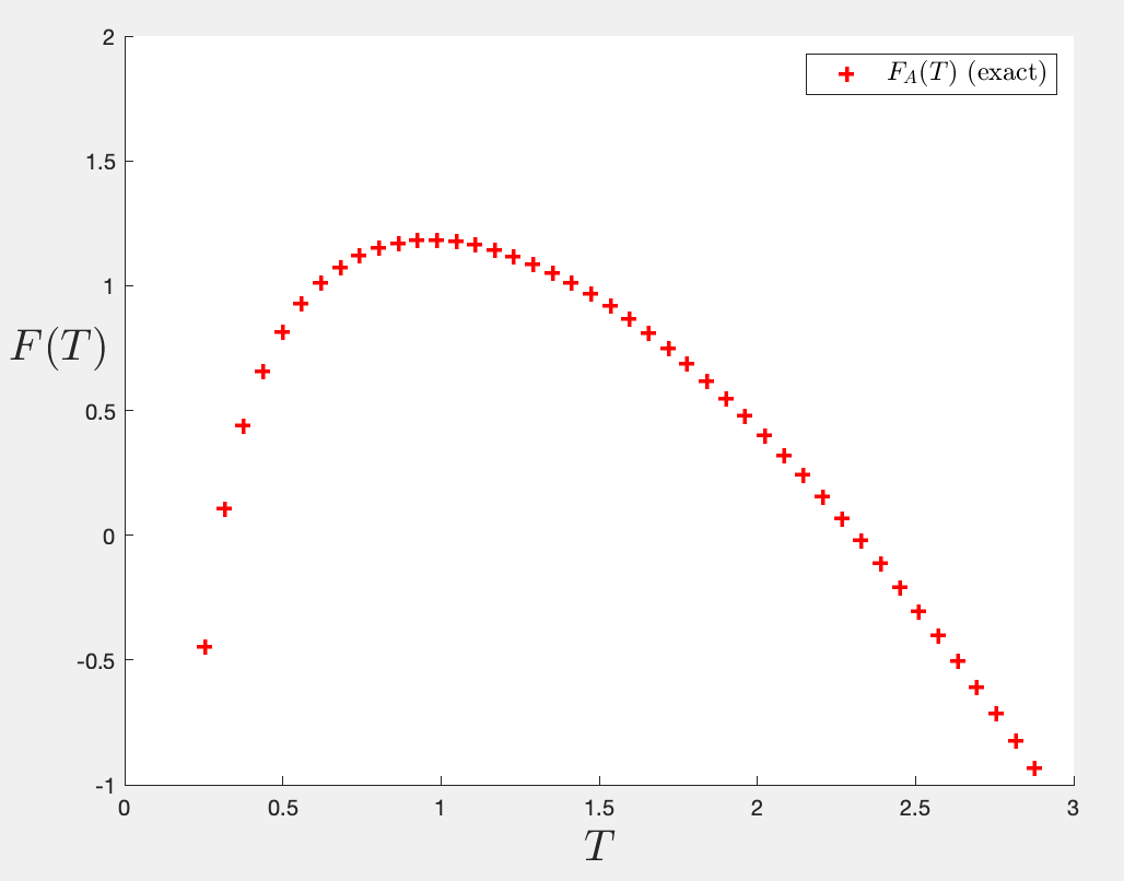
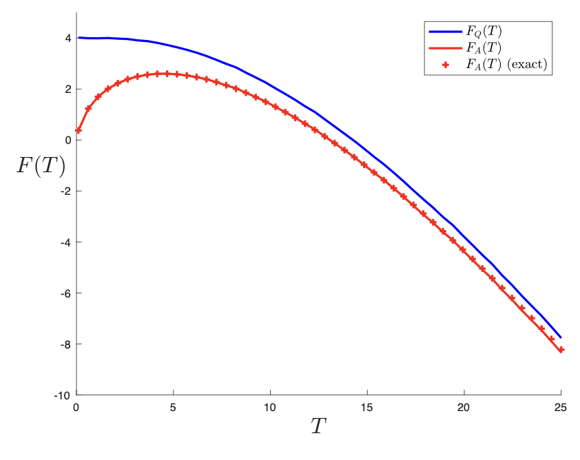
So here’s the punchline. A short while after feeling pleased with myself for the success of this exercise in illustration, I realized that I could do an obvious thing. Since the results line up so nicely from scaling and sampling 100 by 100 matrices, why don’t I just mine the same data set and compute the quenched free energy directly this way?! So obvious. Why had I not thought of this before? (It seems that from the literature, nobody had.) This takes another five minutes to add the right lines of code, and then run a loop to do it over several sample temperatures, and voila!
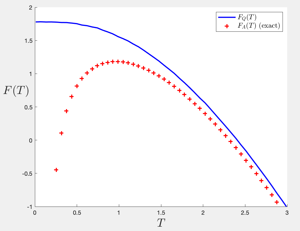
The quenched free energy for the Airy model vs the annealed. The entropy goes nicely to zero!
Some nice things to notice:
- The quenched free energy indeed asymptotes to the annealed free energy at large temperature.
- The entropy (minus the slope of the blue curve) runs nicely to zero at zero temperature, where indeed all that is left is the extremal entropy
- The free energy lands at a special value at zero temperature:
, the average value of the ground state energy. This is nice and also reasonable! The influence of the micro-physics is present in a very natural way!
- It turns out (and this is when I properly began to appreciate the lovely analysis of a recent paper by Janssen and Mirbabayi who did some low temp predictions of this) that the initial fall off from zero temperature looks rather flat, and this is because it goes like
, with a coefficient that is again controlled by the underlying statistics of the microphysics (the distribution of the gap
in fact, worked out by Forrester, Bornemann and Witte, and by Perret and Schehr (References in my paper)). Of course, this way you get more than just the low temperature limit, you get the whole thing.
How lovely to see the whole behaviour for arbitrary temperature come out so nicely!
I won’t go into it here, but this is just the beginning. That large family of Bessel models I described has several nice phenomena that can be studied analytically and laid alongside the numerics. There’s even more wonderful results in the statistical mechanics literature that then show up in the analogous computation of the quenched free energy (that again does not seem to have been done before). For example, the first peak (red) in the Bessel example above turns out to be an exponential (Edelman, Forrester), and the average energy is simply 
Quenched free energy vs the annealed, for the simplest Bessel model.
I could go on about other features, and the numerous other exciting results I got by mining this rich seam of models, but I’ll instead refer you to the paper. (In case you already looked at it, note that there’s a lot of new material (all of this and more) in version 2, and it has a major correction to the overall picture that was painted in v1. It also has a big shout-out to Janssen and Mirbabayi’s very nice recent low T analysis that a lot of my results verify and extend.)
So here’s the big picture thought to wrap up all of this. What was shown above extends to the full matrix models of JT gravity (if you use a stable definition) and variants thereof. (Although it is (so far) hard to generate accurate explicit curves of the sort I showed above for the toy models, see the paper for more on that). I keep emphasizing that this is a fantastic example of the quantum black holes’ (i.e., 4D extremal black holes’) explicit microphysics at play here. The detailed behaviour of the free energy, including its eventual zero temperature value, is all controlled by this microphysics. Without having control of the microphysics in full detail (e.g. by using the matrix model description as I’ve done here, or something equivalent), these features can’t be derived.
What fun!
-cvj

Pingback: Embracing Both Wigner and 't Hooft | Asymptotia
Pingback: Completing a Story | Asymptotia
Pingback: A Return | Asymptotia