Search Results for: JT gravity

Matrices and Gravity

So I have a confession to make. I started working on random matrix models (the large $latex N$, double-scaled variety) in 1990 or 1991, so about 30 years ago, give or take. I’ve written many papers on the topic, some of which people have even read. A subset of those have even been cited from time to time. So I’m supposed to be some kind of expert. I’ve written extensively about them here (search for matrix models and see what comes up), including posts on how exciting they are for understanding aspects of quantum gravity and black holes. So you’d think that I’d actually done the obvious thing right? Actually taken a bunch of random matrices and played with them directly. I don’t mean the fancy path integral formulation we all learn, where you take N large, find saddle points, solve for the Wigner semi-circle law that the Dyson gas of eigenvalues forms, and so forth. I don’t mean the Feynman expansion of that same path integral, and identify (following ‘t Hooft) their topology with a tessellation of random 2D surfaces. I don’t mean the decomposition into orthogonal polynomials, the rewriting of the whole problem at large $latex N$ as a theory of quantum mechanics, and so forth. No, those things I know well. I just mean do what it says on the packet: close your eyes, grab a matrix out of the bag at random, compute its eigenvalues. Then do it again. Repeat a few thousand times and see that all those things in the data that we compute those fancy ways really are true. I realized the other day that in 30 years I’d never actually done that, and (motivated by the desire to make a simple visual illustration of a point) I decided to do it, and it opened up some wonderful vistas.
Let me tell you a little more. […] Click to continue reading this post

Black Holes and a Return to 2D Gravity! – Part II

(A somewhat more technical post follows.)

Continuing from part I: Well, I set the scene there, and so after that, a number of different ideas come together nicely. Let me list them:

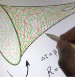
[caption id="attachment_19442" align="alignright" width="250"]illustration of JT gravity background What “nearly” AdS_2 looks like via JT gravity. The boundary wiggles, but has fixed length 1/T.[/caption]
  • Exact solution of the SYK model (or dual JT model) in that low temperature limit I mentioned before gave an answer for the partition function $latex Z(\beta)$, by solving the Schwarzian dynamics for the wiggling boundary that I mentioned earlier. (The interior has a model of gravity on $latex AdS_2$, as I mentioned before, but as we’re in 2D, there’s no local dynamics associated with that part. But we’ll see in a moment that there’s very interesting stuff to take into account there too.) Anyway, the result for the Schwarzian dynamics can be written (see Stanford and Witten) in a way familiar from standard, say, statistical mechanics: $latex Z_0(\beta)=\int dE \rho_0(E) \exp(-\beta E)$, where $latex \rho_0(E)\sim\sinh(2\pi\sqrt{E})$ is the spectral density of the model. I now need to explain why everything has a subscript 0 in it in the last sentence.
  • On the other hand, the JT gravity model organises itself as a very interesting topological sum that is important if we are doing quantum gravity. First, recall that we’re working in the “Euclidean” manner discussed before (i.e., time is a spatial parameter, and so 2D space can be tessellated in that nice Escher way). The point is that the Einstein-Hilbert action in 2D is a topological counting parameter (as mentioned before, there’s no dynamics!). The thing that is being counted is the Euler characteristic of the space: $latex \chi=2-2g-b-c$, where $latex g,b,c$ are the number of handles, boundaries, and crosscaps the surface has, characterising its topology. Forget about crosscaps for now (that has to do with unorientable surfaces like a möbius strip $latex (g=0,b=1,c=1)$ – we’ll stick with orientable surfaces here). The full JT gravity action therefore has just the thing one needs to keep track of the dynamics of the quantum theory, and the partition function (or other quantities that you might wish to compute) can be written as a sum of contributions from every possible topology. So one can write the JT partition function as $latex Z(\beta)=\sum_{g=0}^\infty\hbar^{-(1-2g)}Z_g(\beta)$ where the parameter $latex \hbar$ weights different genus surfaces. In that sum the weight of a surface is $latex \hbar^{-\chi}$ and $latex b=1$ since there’s a boundary of length $latex \beta$, you may recall.

    The basic Schwarzian computation mentioned above therefore gives the leading piece of the partition function, i.e., $latex g=0$, and so that’s why I put the subscript 0 on it at the outset. A big question then is what is the result for JT gravity computed on all those other topologies?!

  • Click to continue reading this post

Black Holes and a Return to 2D Gravity! – Part I

(A somewhat more technical post follows.) Well, I think I promised to say a bit more about what I’ve been up to in that work that resulted in the paper I talked about in an earlier post. The title of my paper, “Non-perturbative JT gravity” has JT (Jackiw-Teitelbiom) gravity in … Click to continue reading this post

A New Distribution

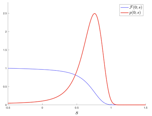
Probability distributionThe red curve in this figure is the probability distribution of the ground state energy [latex]E=s[/latex] of the microstate spectra of quantum completions of JT gravity. Put differently (the way Wigner might have) if you ask what are all the discrete spectra that are compatible with the leading semi-classical result for quantizing JT gravity (the famous Schwarzian result for the density of states: [latex]\rho(E)=e^{S_0}(4\pi^2)^{-1}\sinh(2\pi\sqrt{E})[/latex]), this curve gives the shape of the distribution of ground states. (The blue curve is simply the associated CDF.) I first uncovered this distribution in a paper last year, with further insights and generalizations in a paper earlier this year, along with the distributions for higher energy levels that follow from it. But the exciting new result of my paper from a few weeks ago is that I have now shown that it is a solution of an ordinary differential equation (or a family of them). This allows for some powerful universal things to be said analytically about the properties of the distribution!

This is fully analogous to what happened for the well-known Tracy-Widom distribution for the largest (or smallest) energy of Gaussian random hermitian matrices. While many workers (such as Forrester) had uncovered important aspects of the distribution, and while it was known that it can be expressed as a particular Fredholm determinant, Tracy and Widom broke new ground in 1994 by showing that the distribution was governed by a well known ODE – the Painleve II equation – and in particular can be given in terms of a special solution of it studied earlier by Hastings and McLeod. The result helped forge further connections between properties of random matrix theory and several interesting areas of mathematics and mathematical physics. Furthermore, […] Click to continue reading this post

Completing a Story

[A rather technical post follows.]

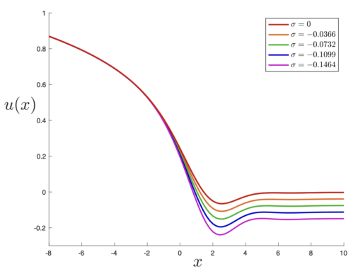
[caption id="attachment_19916" align="aligncenter" width="499"]Sample image from paper. Will be discussed later in the text. This figure will make more sense later in the post. It is here for decoration. Sit tight.[/caption]

For curious physicists following certain developments over the last two years, I’ll put below one or two thoughts about the new paper I posted on the arXiv a few days ago. It is called “Consistency Conditions for Non-Perturbartive Completions of JT Gravity”. (Actually, I was writing a different paper, but a glorious idea popped into my head and took over, so this one emerged and jumped out in front of the other. A nice aspect of this story is that I get to wave back at myself from almost 30 years ago, writing my first paper in Princeton, waving to myself 30 years in the future. See my last post about where I happen to be visiting now.) Anyway here are the thoughts:

Almost exactly two years ago I wrote a paper that explained how to define and construct a non-perturbatively stable completion of JT gravity. It had been defined earlier that year as a perturbative […] Click to continue reading this post

Full Circle

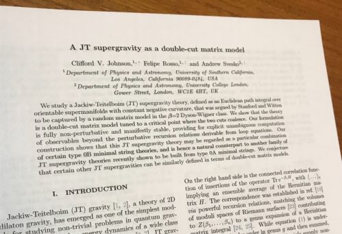
snapshot of paper

Yesterday I submitted (with collaborators Felipe Rosso and Andrew Svesko) a new paper to the arXiv that I’m very excited about! It came from one of those lovely moments when a warm flash of realisation splashed through my mind, and several fragments of (seemingly separate things) that had been floating around in my head for some time suddenly all fit together. The fit was so tight and compelling that I had a feeling of certainty that it just “had to be right”. It is a great feeling, when that happens. Of course, the details had to be worked out, and everything checked and properly developed, new tools made and some very nice computations done to unpack the consequences of the idea… and that’s what resulted in this paper! It is a very natural companion to the cluster of papers I wrote last year, particularly the ones in May and June.

What’s the story? It’s all about Jackiw-Teitelboim (JT) gravity, a kind of 2D gravity theory that shows up rather generically as controlling the low temperature physics of a wide class of black holes, including 4D ones in our universe. Understanding the quantum gravity of JT is a very nice step in understanding quantum properties of black holes. This is exciting stuff!

Ok, now I’ll get a bit more technical. Some background on all this (JT gravity, matrix models, etc), can be found in an earlier pair of posts. You might recall that in May last year I put out a paper where I showed how to define, fully non-perturbatively, a class of Jackiw-Teitelbiom (JT) supergravity theories that had been defined in 2019 in a massive paper by Stanford and Witten (SW). In effect, I showed how to build them as a particular combination of an infinite number of special “minimal string” models called type 0A strings. Those in turn are made using a special class of random matrix model based on […] Click to continue reading this post

Spectral, II

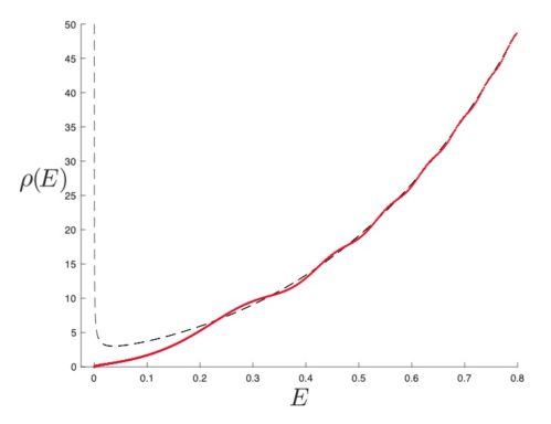
plot of spectral density of (2,2) JT SupergravityWhat’s that now? You want more physics teases? Ok. That dotted line is a (known) JT gravity Schwarzian spectral density. That red line? It’s the fully quantum corrected result! To all orders in topology and beyond. See my paper that appeared today on the arXiv.

(For experts: The red line is made up of about 2000 points for each of which I know the energy, and the full wave function for an associated problem. Using those I can compute lots of things, to good accuracy. One example is the full non-perturbative spectral form factor, that I showed last post.)

-cvj Click to continue reading this post

Multicritical Matrix Model Miracles

Well, that was my title for my seminar last Thursday at the KITP. My plan was to explain more the techniques behind some of the work I’ve been doing over the last few years, in particular the business of treating multicritical matrix models as building blocks for making more complicated theories of gravity.

chalkboard from KITP seminar

The seminar ended up being a bit scattered in places as I realised that I had to re-adjust my ambitions to match limitations of time, and so ended up improvising here and there to explain certain computational details more, partly in response to questions. This always happens of course, and I sort of knew it would at the outset (as was clear from my opening remarks of the talk). The point is that I work on a set of techniques that are very powerful at what they do, and most people of a certain generation don’t know those techniques as they fell out of vogue a long time ago. In the last few years I’ve resurrected them and developed them to a point where they can now do some marvellous things. But when I give talks about them it means I have a choice: I can quickly summarise and then get to the new results, in which case people think I’m performing magic tricks since they don’t know the methods, or I can try to unpack and review the methods, in which case I never get to the new results. Either way, you’re not likely to get people to dive in and help move the research program forward, which should be the main point of explaining your results. (The same problem occurs to some extent when I write papers on this stuff: short paper getting swiftly to the point, or long paper laying out all the methods first? The last time I did the latter, tons of new results got missed inside what people thought was largely just a review paper, so I’m not doing that any more.)

Anyway, so I ended up trying at least to explain what (basic) multicritical matrix models were, since it turns out that most people don’t know these days what the (often invoked) double scaling limit of a matrix model really is, in detail. This ended up taking most of the hour, so I at least managed to get that across, and whet the appetite of the younger people in the audience to learn more about how this stuff works and appreciate how very approachable these techniques are. I spent a good amount of time trying to show how to compute everything from scratch – part of the demystifying process.

I did mention (and worked out detailed notes on) briefly a different class of […] Click to continue reading this post

Embracing Both Wigner and ‘t Hooft

That Feeling

Several weeks ago, while writing up a nice set of results that extended some work I did last year, I found that I was stuck finding the right wording for how I should nuance a (seemingly minor) matter in the introductory remarks. It was partly because, frankly, I’d got bored of the standard introduction I usually make to papers on this particular subject (matrix models and 2D gravity), because I’ve written quite a few in the last two years (10-Yikes!). But I’d found a new feature that warranted a more careful way of saying the usual things, and I wanted to incorporate that aspect, and also get the Reader interested in why this aspect was interesting and worth unpacking. I played around with better ways of saying it, and still was not entirely happy. I chipped away for a bit more over a few days, and kept coming up with something less than satisfactory. I’d carry on with things in the body of the paper that would be there whatever the introduction said. Then, after coming back to the introduction and trying again, I had to stop and explore the consequences of some of the rephrasing I was doing – to make sense of the new way I was trying to say what I wanted to say.

And then it happened…

You might know that feeling: A sort of pop goes off in your head and a tingle through the whole body, and then everything looks different all of a sudden, because you realize that you’ve found a completely new way of looking at things. A way that fits *so* well and incorporates so many of the facts that it just. feels. inevitable.

That’s what happened. And then I tried to see what it would say about the larger picture of physics this all fits in, looking for a way to make it fit, or to challenge the idea to see if it breaks. Not only did not not break, it just kept making sense, and (almost like the idea itself took charge of the process) immediately offered solutions to the problems I threw at it, and readily gobbled up existing challenges that the community has been facing for a while, and explained certain things that have been a puzzle for a long time.

For the next few days I actually could not write properly at the keyboard any more. My hands were trembling every time as I utterly rebuilt the entire paper and my world view, and I could barely sit still at times.

I know this sounds like a lot, and you should know that I am open to the possibility that it is somehow wrong, but it is too compelling not to share, so that’s what my paper that came out earlier this week is all about. I am not going to repeat the paper here, but will try to highlight some features of it that form a foundation for why this changes a lot about how we think about things in this corner of physics.

Random Stuff

Let me start in the simplest way possible, as I have done in the past, with a model that is well known to many different physics communities. The Gaussian random matrix model. Random matrix models have a very long history in trying to understand complicated systems (going back to Wishart (1928), and then Wigner (1955) – physicists seem to always forget to mention Wishart, and I’m sure I’m forgetting someone else too), and they show up in all kinds for systems. There are a lot of powerful results that have been developed, and you’ve read my writings about them here to do with how they get used for understanding aspects of string theory and quantum gravity in 2D, and also in higher dimensions. The “double scaling limit” is something I’ve talked about a lot here in particular. I won’t repeat all of it here, but invite you to go and look at other posts.
[…] Click to continue reading this post