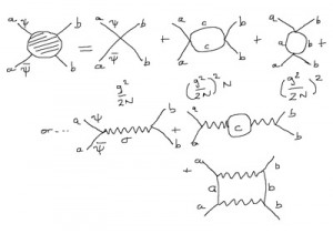
I’ve had a fun time over the last few lectures with some more mature topics, pointing the students to things that they will see more (I hope) in the advanced class next semester.  We covered the large N Gross-Neveu model in some detail, giving me the opportunity to give a glimpse of several important topics and techniques… at large N the 2 dimensional model’s solution is exact, and it shows important phenomena such as spontaneous chiral symmetry breaking, dynamical mass generation for the fermions and dimensional transmutation. These are all important phenomena shared by (the more difficult to study) quantum chromodynamics, the theory of the strong nuclear interactions. (See an earlier post about some of these properties and what they are… there’s also a mention of a new general level book that goes into some detail on the physics and the history.)
The other thing I took some time to explore was the diagrammatics of the model, and the interesting patterns that emerge  when N is large. This is a kind of vector model, where the size (N) of the vectors goes large (there are N quarks in the fundamental of U(N), if you want to be technical… the U(N) is a global symmetry here), and as such the Feynman diagrams organize themselves in such a way that ribbon-like structures are favoured. Matrix models, on the other hand, have a diagrammatic organization in terms of two dimensional surfaces… see an earlier post. When you work at large N, lowest genus (the sphere) is favoured, then the torus, double torus, etc, in an expansion in 1/N. So while field theories of matrices at large N are good for studying random surfaces organized by topology (a powerful tool for understanding formulations of string theory, actually), field theories of vectors at large N are good for the study of random strand-like structures, like polymers. Large N favours fewer branchings…
Anyway, I wish I could have gone on more about such things, but time is short. There’s only one more lecture left, and so I’ll be wrapping things up shortly. It was a great class to teach.
-cvj


Ha ha! Thank you. I will look at it. But I fear this is so different from our math, we won’t connect it for a while. Even your equation is another funny drawing, admittedly, with more familiar characters.
Hi,
No. I’ve made hand-written notes from various sources (e.g. Coleman, Zee, etc), but they are not available. The original papers and those texts are excellent sources though.
Cheers,
-cvj
Awesome Clifford. I really would have loved to be able to take that class with you. (Ive been teaching myself a lot of QFT, but its not quite the same without the pressure of grades hanging over your head…)
Do you happen to have any good pdf notes or anything on this particular model?
🙂
All starts with this post: http://asymptotia.com/2011/09/02/laying-down-the-lines/
Look in the image of all the diagrams…and the explanation… they represent the leading terms in a small [tex]\lambda[/tex] expansion of (part of) the expressions in the top left hand part… which in turn represent the integral:
[tex]Z(J)=\int_{-\infty}^{+\infty}d\phi\, e^{-\frac12 m^2 \phi^2 {-} \frac{\lambda}{4!}\phi^4+J\phi},[/tex]
which has the structure of a quantum field theory, used to describe interacting elementary particles (for example) but simplified a tad. (It is in 0+0 dimensions in this example… you can add stuff that makes for propagation in space and time which means a bit more work on each diagram, but the diagrams themselves are structurally the same….)
-cvj
I’ve taken to printing some of these images and putting them with my math notebook. Then I show them to my friends at Discrete Mathematics Class and we gawk over what they might mean.