Landmarks

We reached certain key landmarks in the quantum field theory class last week. Not only did we uncover how the Dirac equation predicts that the electron’s spin couples to a background magnetic field, but that it is (to a first approximation) twice the coupling that its angular momentum couples with. This is a remarkable output (once again) from that wonderful equation, the result of putting together Quantum Mechanics and Special Relativity. (I’ve discussed other properties of it before, here.) Makes you wonder, doesn’t it? If finding an equation that puts together QM and SR results in so many marvellous things about Nature just falling out so nicely (recall that spin, and also antimatter are also inevitable predictions of the Dirac equation), doesn’t it make you just thirst to know what we’ll learn (predict, explain, discover) when we find how Quantum Mechanics and General Relativity fit together? This is one of the great motivations for the work my research community does, in case you sometimes find yourself wondering – the quest for finding how Nature combines the two things together to make what we call Quantum Gravity. We’ve found one way, on the page, that you can put together QM and GR for sure (you’ve heard of it, it is called string theory) but it’s not yet clear if this form of quantum gravity is the one Nature chooses to work with, and in any case we need to work on it a lot more to understand what we’ve got, as it surely isn’t complete yet. There are huge pieces of the puzzle missing.

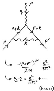
Anyway, the next thing we did was the classic computation of the first quantum correction to the “twice” I mentioned above. This is the computation of the famous “g-2” for the electron (“anomalous magnetic moment” is also a term sometimes used, in case you’re going to google). The symbol “g” is the ratio of coupling strengths, and it is not quite 2, but slightly different from 2. That tiny number is what needs to be computed from first principles using quantum electrodynamics (QED). It is often quoted as the most accurately experimentally verified computation in the history of science, and not without justification, since it involves an accuracy down to the 12th or 13th digit after the decimal point. (Better than the specifying the distance between New York and Los Angeles to an accuracy better than the thickness of a human hair, an analogy that Feynman used to electrify young budding physicists in his little book QED a long time ago).

I spent one of my train journeys to Santa Barbara carefully isolating all the details in the computation (just the part that gets the first four or five digits right) so that we could see it all in class in all its glory. In the language of diagrams I showed you some posts ago, it all boils down to extracting the right pieces of computation represented by the diagram above left. It was fun to work through it with the students…